Determination of Income and Employment – Class 12 Economics Notes
Part B: Introductory Macroeconomics
Chapter – 4
Determination of Income and Employment
This chapter explains how the equilibrium level of income (output) and employment is determined in the short run, assuming the price level is fixed and there is unemployment (so output can rise to meet demand). The analysis follows J. M. Keynes, and assumes a two-sector economy (households and firms) unless stated otherwise.
4.1 Aggregate Demand and its Components
Aggregate demand (AD) is the total planned (ex-ante) expenditure on final goods and services in an economy during a period. In a two-sector economy, AD = C + I (in a four-sector economy, AD = C + I + G + (X – M)). Aggregate supply (AS) is the total value of output planned to be produced; it equals national income: AS = C + S = Y.
Ex-ante means planned (intended) values; ex-post means actual (realised) values. Ex-post saving always equals ex-post investment, but ex-ante saving and investment may differ.
4.1.1 Consumption
Consumption function (propensity to consume): the relationship between consumption and income. Keynes’s simple linear form: C = C̄ + bY, where C̄ (> 0) is autonomous consumption (consumption even at zero income) and b is the marginal propensity to consume (MPC), 0 < b < 1. The saving function is S = Y – C = -C̄ + (1 – b)Y.
Concept | Formula | Meaning |
|---|---|---|
APC | C/Y | Consumption per unit of income |
MPC | ΔC/ΔY | Change in consumption per unit change in income |
APS | S/Y | Saving per unit of income |
MPS | ΔS/ΔY | Change in saving per unit change in income |
Relations: APC + APS = 1; MPC + MPS = 1. MPC lies between 0 and 1. APC can be greater than 1 at low incomes (when consumption exceeds income, saving is negative), and APC falls as income rises. At the break-even point C = Y, S = 0 and APC = 1.
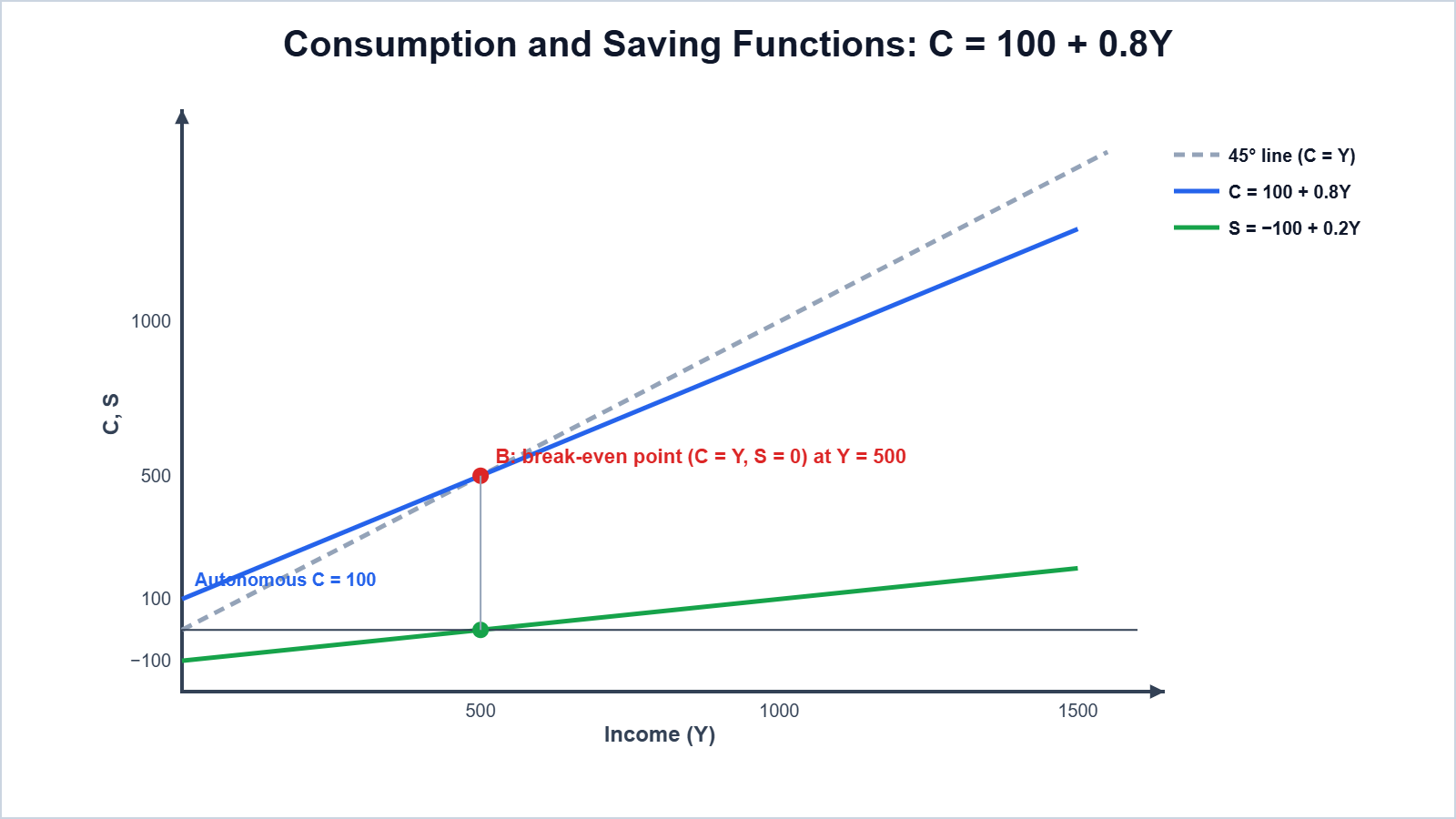
Numerical 1: C = 100 + 0.8Y. Find consumption and saving at Y = 0, 500, 1000 and 1500.
Given: C̄ = 100; b = 0.8
Formula: C = 100 + 0.8Y; S = Y – C
Solution: Y = 0: C = 100, S = -100. Y = 500: C = 500, S = 0. Y = 1000: C = 900, S = 100. Y = 1500: C = 1300, S = 200
Answer: C = 100, 500, 900, 1300; S = -100, 0, 100, 200; break-even income = 500.
Numerical 2: Using Numerical 1, calculate APC, APS at Y = 1000 and MPC, MPS when Y rises from 1000 to 1500.
Given: At Y = 1000: C = 900, S = 100. At Y = 1500: C = 1300
Formula: APC = C/Y; APS = S/Y; MPC = ΔC/ΔY; MPS = 1 – MPC
Solution: APC = 900/1000; APS = 100/1000; MPC = (1300 – 900)/(1500 – 1000) = 400/500
Answer: APC = 0.9; APS = 0.1; MPC = 0.8; MPS = 0.2
Numerical 3: Income rises 0, 100, 200, 300, 400 and consumption is 40, 120, 200, 280, 360. Find MPC and APC.
Given: Y and C as given
Formula: MPC = ΔC/ΔY; APC = C/Y
Solution: MPC = 80/100 at each step; APC = 120/100, 200/200, 280/300, 360/400
Answer: MPC = 0.8 (constant); APC = 1.2, 1, 0.93, 0.9 (falling)
4.1.2 Investment
Investment is the addition to the stock of physical capital (machines, buildings, roads) and to inventories during a period. In this simple model, investment is taken as autonomous: I = Ī, determined by factors other than income (interest rate, expectations, technology), so its curve is a horizontal line.
4.2 Determination of Income in Two-sector Model
In a two-sector economy, planned output is sold either to consumers or to firms (as investment). Planned expenditure is AD = C̄ + bY + Ī. Equilibrium requires planned output (Y) to equal planned expenditure (AD).
4.3 Determination of Equilibrium Income in the Short Run
4.3.1 Macroeconomic Equilibrium with Price Level Fixed
AD-AS approach: equilibrium is where Y = AD, i.e., where the AD line cuts the 45° line. Y* = (C̄ + Ī) / (1 – b).

If AD > AS (to the left of E), demand exceeds output, inventories fall, and producers raise output. If AD < AS (right of E), unplanned stocks pile up and output is cut. So the economy moves to E.
Saving-investment approach: equilibrium is where planned saving = planned investment (S = I). Since Y = C + S and AD = C + I, Y = AD means S = I.

Numerical 4: C = 100 + 0.8Y and I = 100. Find the equilibrium income, consumption and saving.
Given: C̄ = 100; b = 0.8; Ī = 100
Formula: Y* = (C̄ + Ī)/(1 – b)
Solution: Y* = (100 + 100)/0.2 = 1000; C = 100 + 800 = 900; S = 1000 – 900
Answer: Y* = 1,000; C = 900; S = 100 = I (both approaches agree)
Numerical 5: C = 200 + 0.75Y and equilibrium income is 2,000. Find investment.
Given: C̄ = 200; b = 0.75; Y = 2000
Formula: At equilibrium S = I, where S = Y – C
Solution: C = 200 + 0.75 x 2000 = 1700; S = 2000 – 1700
Answer: I = 300
4.3.2 Effect of an Autonomous Change in Aggregate Demand on Income and Output
An increase in autonomous expenditure (for example, a rise in Ī by ΔI, or in C̄) shifts the AD line up in parallel. The new equilibrium income rises by more than the increase in autonomous expenditure.
4.3.3 The Multiplier Mechanism
Investment multiplier (k) = ΔY/ΔI = 1/(1 – MPC) = 1/MPS. The process: an increase in investment of ΔI raises incomes of producers by ΔI; they spend MPC x ΔI, which becomes others’ income; they spend MPC2 x ΔI, and so on. Total ΔY = ΔI(1 + b + b2 + …) = ΔI/(1 – b).
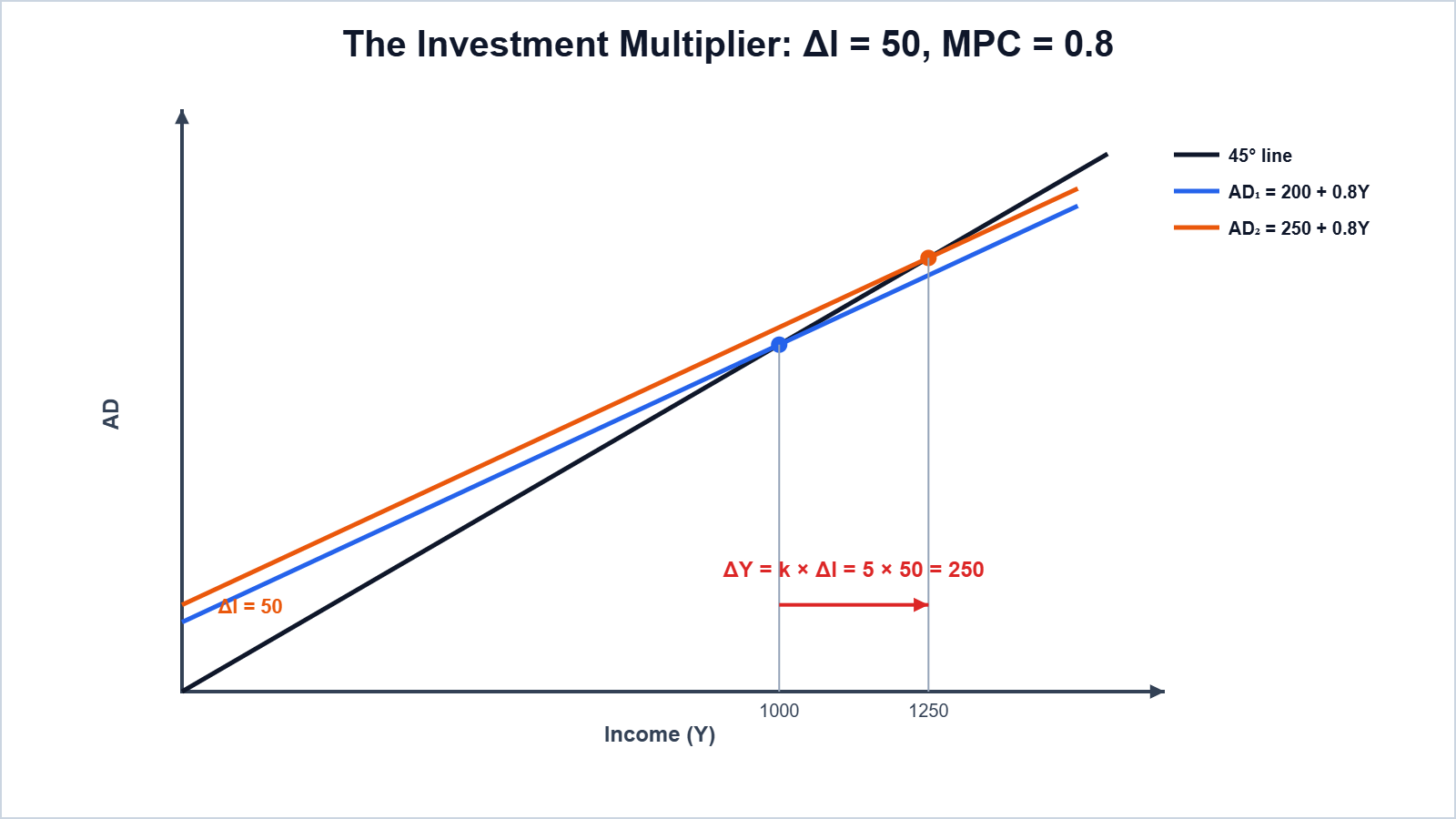
Numerical 6: MPC = 0.8 and investment rises by ₹50 crore. Find the multiplier and the increase in income.
Given: MPC = 0.8; ΔI = 50
Formula: k = 1/(1 – MPC); ΔY = k x ΔI
Solution: k = 1/0.2 = 5; ΔY = 5 x 50
Answer: k = 5; ΔY = ₹250 crore (income rises from 1,000 to 1,250 in the model above)
Numerical 7: MPS = 0.25. How much should investment increase to raise income by ₹1,000 crore?
Given: MPS = 0.25; ΔY = 1000
Formula: k = 1/MPS; ΔI = ΔY/k
Solution: k = 1/0.25 = 4; ΔI = 1000/4
Answer: ΔI = ₹250 crore
MPC | MPS | Multiplier |
|---|---|---|
0.5 | 0.5 | 2 |
0.75 | 0.25 | 4 |
0.8 | 0.2 | 5 |
0.9 | 0.1 | 10 |
Remember: the multiplier is larger when MPC is larger. Minimum value of k is 1 (MPC = 0) and maximum is infinity (MPC = 1).
4.4 Some More Concepts
Full employment: a situation in which all those willing and able to work at the prevailing wage get work. Involuntary unemployment: people willing to work at the prevailing wage cannot find work. Voluntary unemployment: people choose not to work at the prevailing wage.
Deficient demand and deflationary gap: if AD at full employment output (YF) is less than YF, the shortfall is the deflationary gap. It leads to falling output and employment (unemployment). Excess demand and inflationary gap: if AD at YF exceeds YF, the excess is the inflationary gap; output cannot rise further, so prices rise.
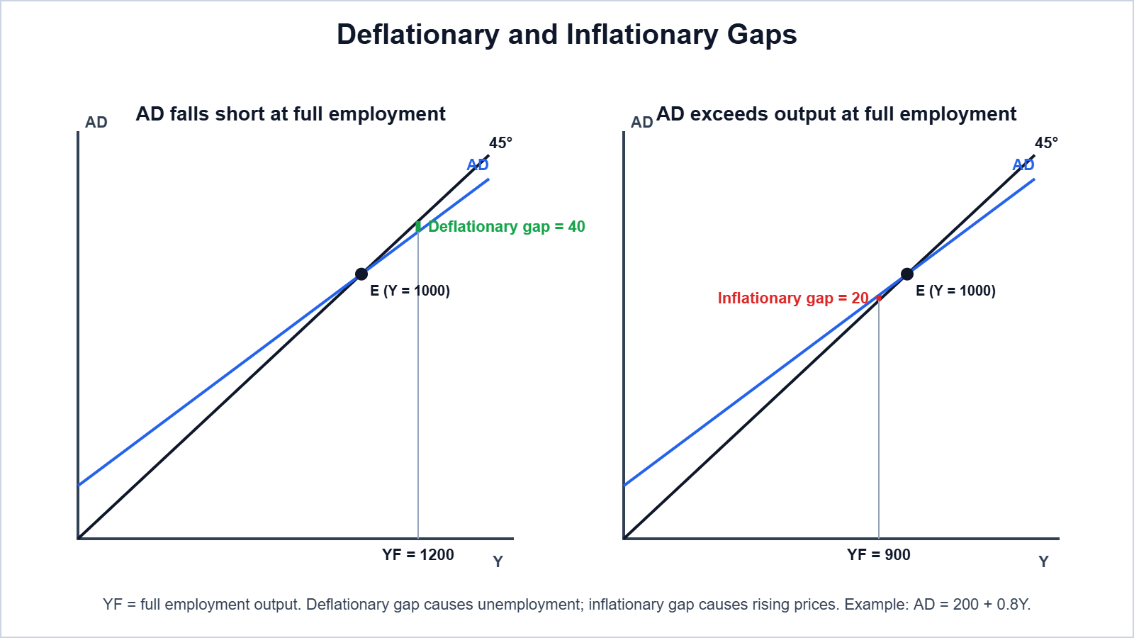
Numerical 8: AD = 200 + 0.8Y (C = 100 + 0.8Y, I = 100). Find the gap if full employment income is (a) 1,200 and (b) 900. By how much must investment change to remove the gap in (a)?
Given: AD = 200 + 0.8Y; equilibrium Y = 1000
Formula: Gap = AD at YF – YF; required ΔY = k x ΔI
Solution: (a) AD at 1200 = 200 + 960 = 1160; gap = 1200 – 1160 = 40. ΔY needed = 1200 – 1000 = 200; ΔI = 200/5 = 40. (b) AD at 900 = 200 + 720 = 920; gap = 920 – 900 = 20
Answer: (a) Deflationary gap = 40, removed by a rise of 40 in investment; (b) inflationary gap = 20
Measures to correct: for a deflationary gap – increase government spending, reduce taxes, lower repo rate/CRR, buy securities (OMO). For an inflationary gap – the opposite measures.
Paradox of thrift: if all households try to save more (raise MPS or reduce autonomous consumption), AD falls, income falls, and total saving does not increase – it may stay the same or even fall. What is good for an individual (saving more) can be harmful for the economy as a whole when there is unemployment.

Numerical 9: C = 100 + 0.8Y and I = 100. Households become thrifty and autonomous consumption falls to 80. Find the new equilibrium income and saving.
Given: C̄ falls from 100 to 80; b = 0.8; I = 100
Formula: Y* = (C̄ + Ī)/(1 – b); S = Y – C
Solution: Y* = (80 + 100)/0.2 = 900; C = 80 + 0.8 x 900 = 800; S = 900 – 800
Answer: Y falls from 1,000 to 900, but saving stays at 100 (= I): the paradox of thrift.
Easy Memory Trick: “k = 1 over MPS”; and “Saving more, earning less” for the paradox of thrift.
Practice Problems (Answers Only)
- MPC = 0.9. Find the multiplier. Ans: 10
- C = 50 + 0.75Y, I = 150. Find equilibrium income. Ans: 800
- k = 5 and ΔY = 500. Find ΔI. Ans: 100
- MPC = 0.6. Find MPS. Ans: 0.4
- If S = -50 + 0.2Y, find the break-even income. Ans: 250
Important Questions
Q1. What is aggregate demand? State its components.
Ans. Total planned expenditure; AD = C + I + G + (X – M) (C + I in a two-sector economy).
Q2. Distinguish between ex-ante and ex-post.
Ans. Ex-ante means planned; ex-post means actual or realised.
Q3. Define MPC and MPS. What is their sum?
Ans. MPC = ΔC/ΔY; MPS = ΔS/ΔY; MPC + MPS = 1.
Q4. Can APC be greater than one? When?
Ans. Yes, at low incomes below the break-even point, when consumption exceeds income.
Q5. Explain the determination of equilibrium income by the AD-AS approach.
Ans. Equilibrium is where AD = AS (the AD line cuts the 45° line); any gap causes changes in stocks and output.
Q6. Explain the S = I approach to equilibrium.
Ans. Equilibrium is where planned saving equals planned investment.
Q7. What is the investment multiplier? Write its formula.
Ans. The ratio of change in income to change in investment: k = 1/(1 – MPC).
Q8. What is a deflationary gap? How can it be corrected?
Ans. Shortfall of AD below full employment output; corrected by raising spending, cutting taxes or easing monetary policy.
Q9. What is an inflationary gap?
Ans. Excess of AD over full employment output, causing a rise in prices.
Q10. Explain the paradox of thrift.
Ans. An attempt by all to save more lowers AD and income, so total saving does not rise.
Conclusion: With prices fixed, equilibrium income is where AD = AS (or S = I). Changes in autonomous spending change income by a multiple through the multiplier k = 1/(1 – MPC), while deflationary and inflationary gaps show deficient and excess demand at full employment.