The Theory of the Firm under Perfect Competition – Class 12 Economics Notes
Part A: Introductory Microeconomics
Chapter – 4
The Theory of the Firm under Perfect Competition
4.1 Perfect Competition: Defining Features
- Large number of buyers and sellers: no single buyer or seller can influence the market price.
- Homogeneous product: output of every firm is identical, so buyers do not prefer any one seller.
- Free entry and exit of firms.
- Perfect information: all buyers and sellers know the market price and conditions.
- Perfect mobility of factors of production.
Result: every firm is a price taker. It can sell any quantity at the market price but nothing at a higher price. Its demand curve is horizontal (perfectly elastic) at the market price.
4.2 Revenue
- Total revenue (TR) = p x q.
- Average revenue (AR) = TR/q = p.
- Marginal revenue (MR) = ΔTR/Δq; under perfect competition MR = p.
So under perfect competition p = AR = MR; the TR curve is a straight line from the origin whose slope equals the price.
Numerical 1: A firm sells at a market price of ₹10. Find TR, AR and MR for outputs 1 to 5.
Given: p = ₹10; q = 1 to 5
Formula: TR = p x q; AR = TR/q; MR = TRq – TRq-1
Solution: TR = 10, 20, 30, 40, 50; AR = 10/1, 20/2, …; MR = 10 – 0, 20 – 10, …
Answer: TR = 10, 20, 30, 40, 50; AR = MR = ₹10 at every output
4.3 Profit Maximisation
Profit (π) = TR – TC. A firm chooses the output q0 that maximises profit. Under perfect competition three conditions must hold:
4.3.1 Condition 1: p = MC at q0 (MR = MC). If p > MC, producing one more unit adds more to revenue than to cost, so output should rise; if p < MC, output should fall.
4.3.2 Condition 2: MC must be non-decreasing (rising) at q0. If MC is falling where p = MC, producing a little more raises profit, so that point is not the maximum.
4.3.3 Condition 3: in the short run, p ≥ AVC at q0 (otherwise the firm should shut down); in the long run, p ≥ AC (LRAC).
4.3.4 The Profit Maximisation Problem: Graphical Representation
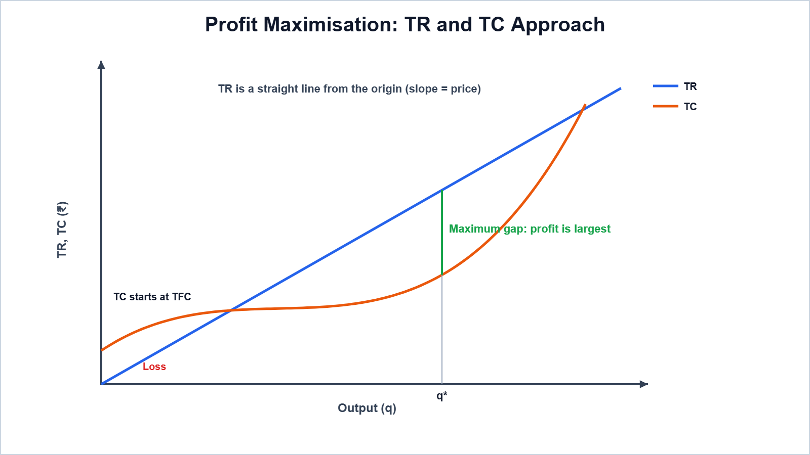
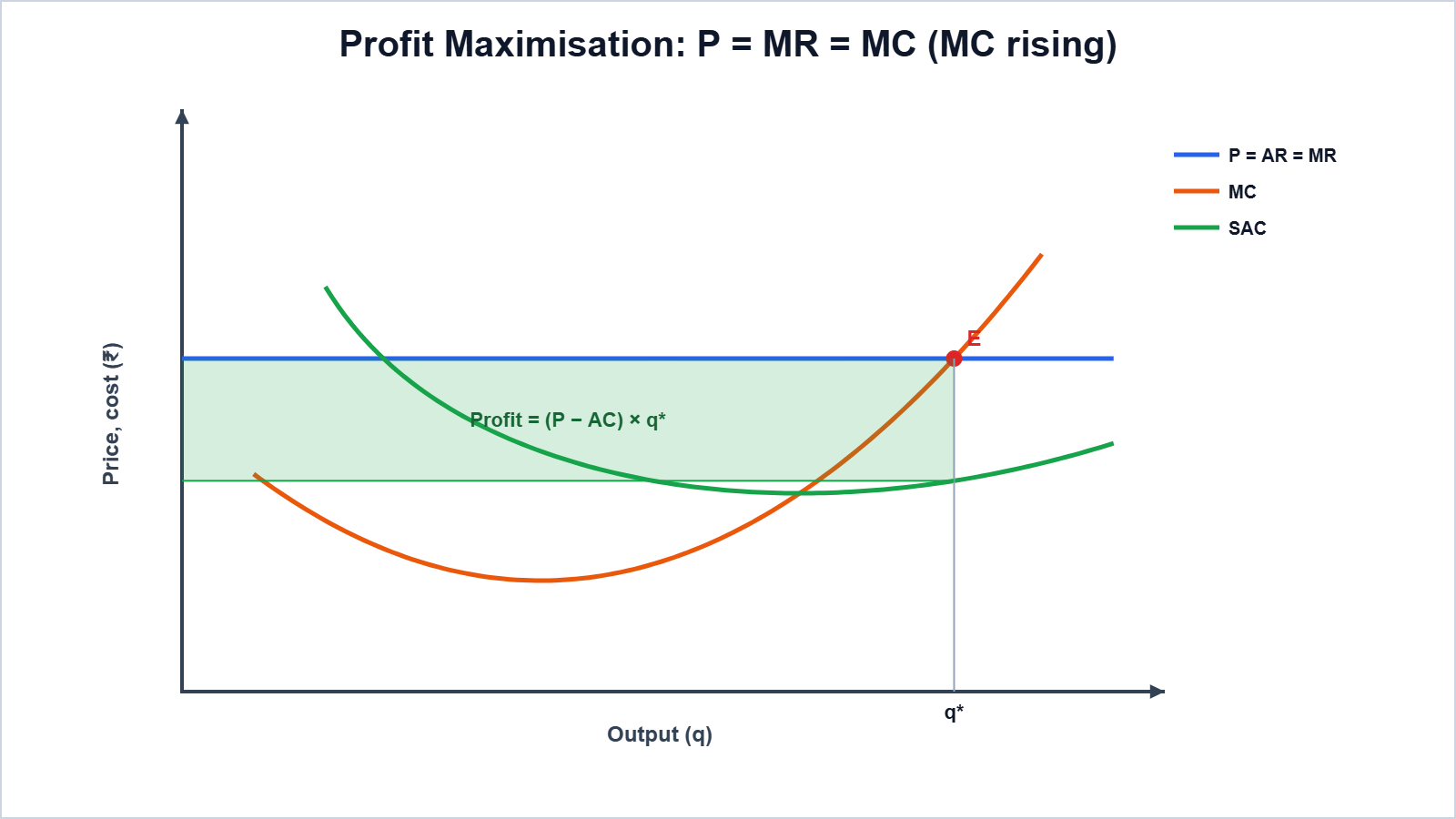
In the second diagram, at E price equals MC on the rising part of MC; profit = (p – AC) x q0 (shaded area). If p were below AC, the same rectangle would show a loss.
q | TR (p = ₹10) | TC | Profit = TR – TC | MR | MC |
|---|---|---|---|---|---|
0 | 0 | 12 | -12 | – | – |
1 | 10 | 18 | -8 | 10 | 6 |
2 | 20 | 22 | -2 | 10 | 4 |
3 | 30 | 25 | 5 | 10 | 3 |
4 | 40 | 30 | 10 | 10 | 5 |
5 | 50 | 38 | 12 | 10 | 8 |
6 | 60 | 50 | 10 | 10 | 12 |
Numerical 2: Price is ₹10 and TC for 0 to 6 units is 12, 18, 22, 25, 30, 38, 50. Find the profit-maximising output by (a) the TR-TC method and (b) the MR-MC method.
Given: p = MR = ₹10; TC as given
Formula: (a) Maximise TR – TC; (b) produce while MR ≥ MC, with MC rising
Solution: (a) Profit = -12, -8, -2, 5, 10, 12, 10, maximum at q = 5. (b) MC = 6, 4, 3, 5, 8, 12: MC ≤ MR up to the 5th unit (8 < 10) but the 6th unit costs 12 > 10
Answer: Profit-maximising output = 5 units; maximum profit = ₹12 (both methods agree)
Remember: in a schedule, MC rarely equals MR exactly; the firm produces up to the last unit for which MC ≤ MR, provided MC is rising after that.
4.4 Supply Curve of a Firm
The supply curve of a firm shows the quantity it will produce at each market price, other things constant.
4.4.1 Short Run Supply Curve of a Firm: for prices at or above minimum AVC, the firm produces where p = MC (rising). For prices below minimum AVC, it produces zero. So the short run supply curve is the rising part of the SMC curve at and above minimum AVC, plus zero output for lower prices.

4.4.2 Long Run Supply Curve of a Firm: in the long run the firm produces where p = LRMC (rising) only if p ≥ minimum LRAC. The long run supply curve is the rising part of LRMC at and above minimum LRAC.
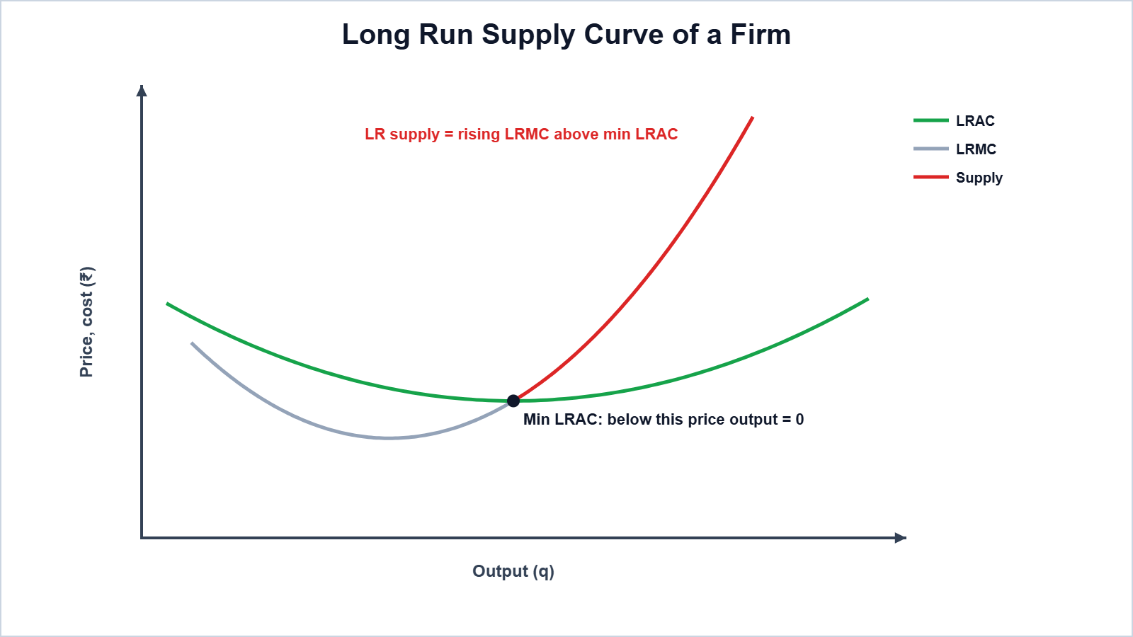
4.4.3 The Shut Down Point: in the short run, a firm continues to produce as long as price covers AVC, because TFC must be paid even if it stops. If p < minimum AVC, it shuts down. The point where p = minimum AVC is the short run shut-down point. In the long run the shut-down point is the minimum of LRAC.
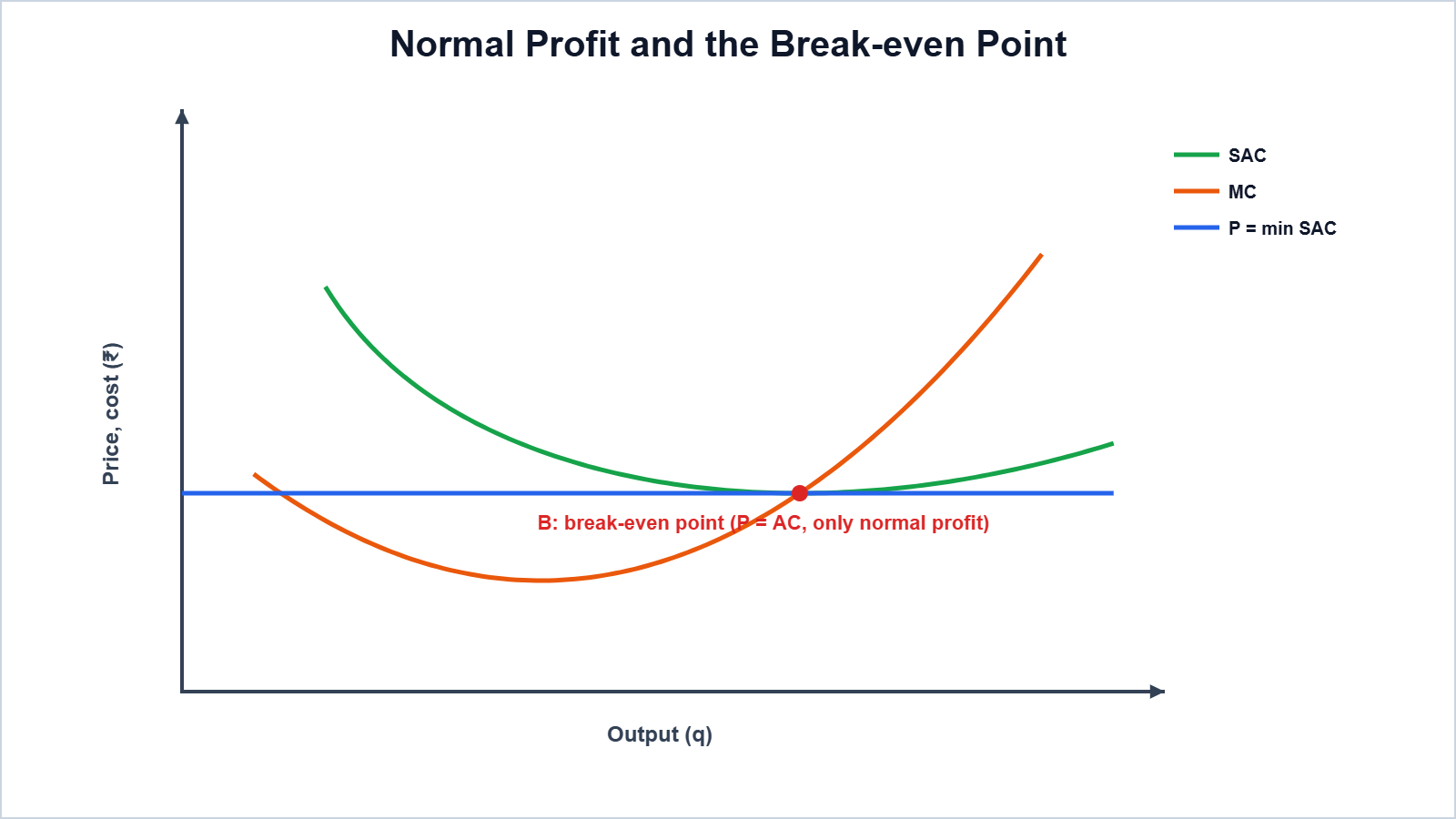
4.4.4 The Normal Profit and Break-even Point: normal profit is the minimum profit needed to keep a firm in business; it is included in costs (as the opportunity cost of the entrepreneur). Profit above normal profit is super-normal (economic) profit. The break-even point is where p = minimum AC: TR = TC and the firm earns only normal profit.
q | TFC | TVC | TC | AVC | AC | MC |
|---|---|---|---|---|---|---|
1 | 24 | 10 | 34 | 10 | 34 | 10 |
2 | 24 | 16 | 40 | 8 | 20 | 6 |
3 | 24 | 24 | 48 | 8 | 16 | 8 |
4 | 24 | 36 | 60 | 9 | 15 | 12 |
5 | 24 | 55 | 79 | 11 | 15.8 | 19 |
Numerical 3: From the cost schedule above, find the shut-down price and the break-even price.
Given: TFC = ₹24; TVC = 10, 16, 24, 36, 55
Formula: Shut-down price = minimum AVC; break-even price = minimum AC
Solution: AVC = 10, 8, 8, 9, 11, minimum = 8; AC = 34, 20, 16, 15, 15.8, minimum = 15
Answer: Shut-down price = ₹8; break-even price = ₹15
Numerical 4: In the schedule above, the market price is ₹12. How much will the firm produce? Will it make a profit or a loss, and should it continue in the short run?
Given: p = ₹12; MC = 10, 6, 8, 12, 19
Formula: p = MC with MC rising; profit = TR – TC; continue if p ≥ AVC
Solution: p = MC = 12 at q = 4 (MC rising). TR = 12 x 4 = 48; TC = 60; profit = 48 – 60. AVC at q = 4 is 9 < 12
Answer: q = 4; loss = ₹12. It should continue in the short run because p > AVC: the loss (₹12) is less than the loss of TFC (₹24) it would suffer by shutting down.
4.5 Determinants of a Firm’s Supply Curve
4.5.1 Technological Progress: better technology raises output from the same inputs, lowers MC and shifts the supply curve to the right.
4.5.2 Input Prices: a rise in input prices (e.g., wages, raw materials) raises MC and shifts the supply curve to the left; a fall shifts it to the right. A unit tax has the same effect as a rise in costs (leftward shift).

4.6 Market Supply Curve
Market supply at a price is the sum of the quantities supplied by all firms at that price. The market supply curve is the horizontal summation of the supply curves of individual firms. It also shifts when the number of firms changes.
Numerical 5: At prices ₹1, 2, 3, 4, firm A supplies 0, 2, 4, 6 units and firm B supplies 0, 1, 2, 3 units. Find the market supply.
Given: qA = 0, 2, 4, 6; qB = 0, 1, 2, 3
Formula: Market supply = qA + qB
Solution: 0 + 0; 2 + 1; 4 + 2; 6 + 3
Answer: Market supply = 0, 3, 6, 9 units
4.7 Price Elasticity of Supply
Price elasticity of supply (eS) = percentage change in quantity supplied / percentage change in price = (ΔQ/ΔP) x (P/Q). It is positive because of the direct relation between price and quantity supplied.
Numerical 6: Price rises from ₹10 to ₹12 and quantity supplied rises from 100 to 130 units. Find eS.
Given: P = 10, P1 = 12, Q = 100, Q1 = 130
Formula: eS = %ΔQ / %ΔP
Solution: %ΔQ = 30/100 x 100 = 30%; %ΔP = 2/10 x 100 = 20%; eS = 30/20
Answer: eS = 1.5 (elastic supply)
Numerical 7: The supply function is q = -10 + 5p. Find eS at p = ₹4.
Given: q = -10 + 5p; ΔQ/ΔP = 5; at p = 4, q = -10 + 20 = 10
Formula: eS = (ΔQ/ΔP) x (P/Q)
Solution: eS = 5 x 4/10
Answer: eS = 2 (the line meets the price axis, so eS > 1, as expected)
Numerical 8: eS of a good is 0.5. If its price rises by 20%, find the new quantity supplied when the initial supply is 200 units.
Given: eS = 0.5; %ΔP = 20%; Q = 200
Formula: %ΔQ = eS x %ΔP
Solution: %ΔQ = 0.5 x 20 = 10%; new Q = 200 + 10% of 200
Answer: 220 units
Geometric method: for a straight-line supply curve, if it meets the price axis eS > 1; if it passes through the origin eS = 1; if it meets the quantity axis eS < 1. A vertical supply curve has eS = 0 and a horizontal one has eS = ∞.
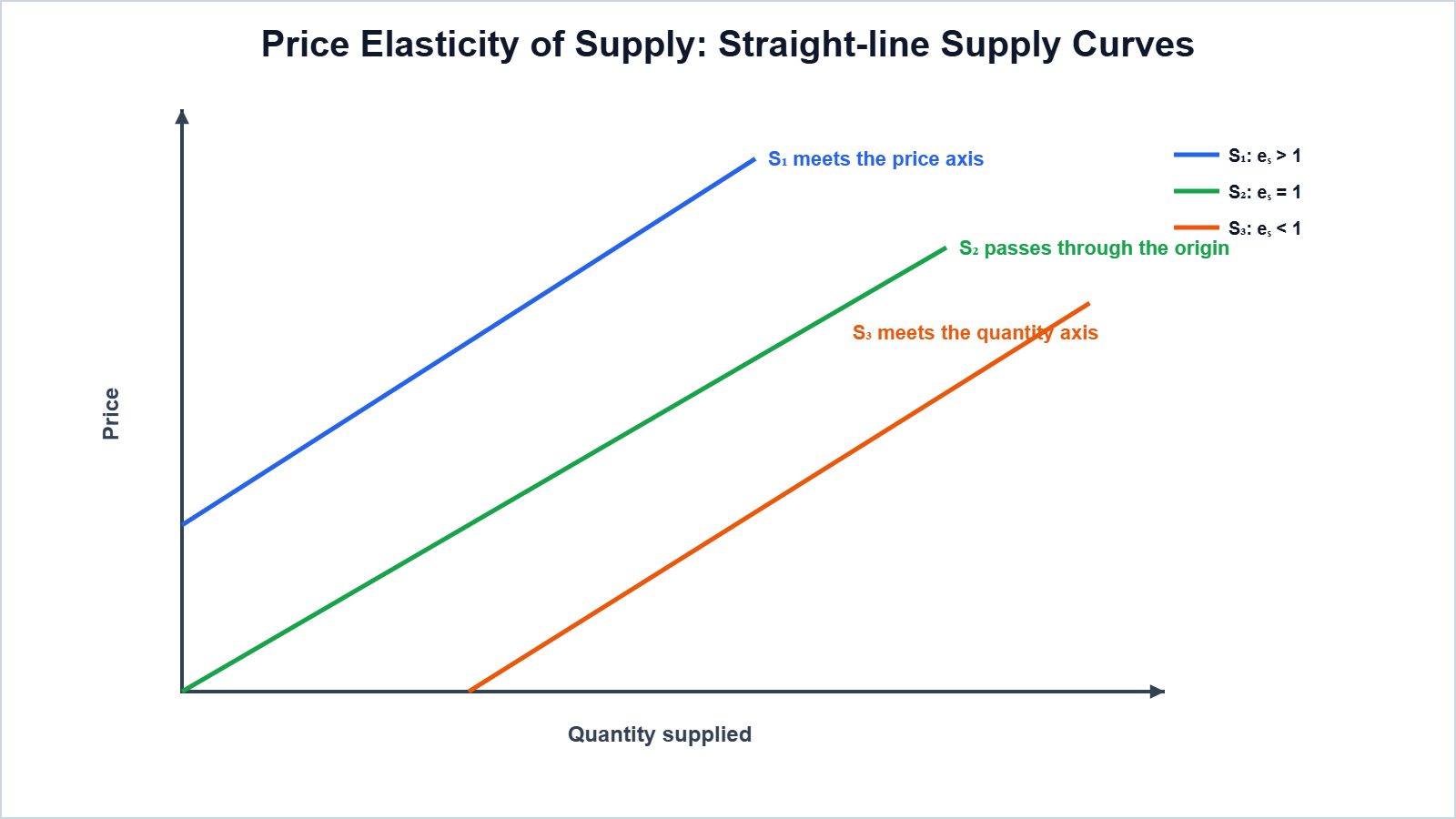
Easy Memory Trick: “P-axis = Plus (more than 1), Origin = One, Q-axis = Quiet (less than 1)”.
Practice Problems (Answers Only)
- A firm sells 8 units at ₹5 each. Find TR, AR and MR. Ans: TR = ₹40; AR = MR = ₹5
- Price rises from ₹5 to ₹6 and supply from 50 to 60 units. Find eS. Ans: 1 (unitary)
- Minimum AVC is ₹20 and market price is ₹18. What will the firm do in the short run? Ans: Shut down (produce zero)
- Minimum AC is ₹30 and price is ₹30. What profit does the firm earn? Ans: Only normal profit (break-even)
- Supply curve q = 2p passes through the origin. Find eS. Ans: 1
Important Questions
Q1. State the features of perfect competition.
Ans. Many buyers and sellers, homogeneous product, free entry and exit, perfect knowledge and perfect factor mobility.
Q2. Why is a firm under perfect competition a price taker?
Ans. Each firm is too small to influence the price, and products are identical.
Q3. Why is AR = MR under perfect competition?
Ans. Price is constant for every unit sold, so each extra unit adds exactly the price to TR.
Q4. State the conditions of profit maximisation.
Ans. p = MC; MC non-decreasing at that output; p ≥ AVC in the short run (p ≥ AC in the long run).
Q5. What is the shut-down point?
Ans. The point where price equals minimum AVC in the short run (minimum LRAC in the long run).
Q6. What is the break-even point?
Ans. The point where price equals minimum AC; TR = TC and only normal profit is earned.
Q7. Why does a firm produce in the short run even at a loss?
Ans. If price covers AVC, it loses less by producing than by shutting down (when the loss would equal TFC).
Q8. Explain two determinants of a firm’s supply curve.
Ans. Technological progress shifts it right; a rise in input prices shifts it left.
Q9. Define price elasticity of supply.
Ans. The percentage change in quantity supplied divided by the percentage change in price.
Q10. What is the elasticity of a supply curve passing through the origin?
Ans. Unity (eS = 1).
Conclusion: A competitive firm, as a price taker, maximises profit where price equals rising MC, provided price covers AVC (short run) or AC (long run). These rules give the firm’s supply curve, and adding the supply of all firms gives the market supply curve.