Theory of Consumer Behaviour – Class 12 Economics Notes
Part A: Introductory Microeconomics
Chapter – 2
Theory of Consumer Behaviour
A consumer buys goods and services to satisfy wants. This chapter studies how a rational consumer chooses the best affordable bundle of goods, and how demand arises from this choice.
2.1 Utility
Utility is the want-satisfying power of a commodity. It is subjective: the same good gives different utility to different people, and to the same person at different times or places.
2.1.1 Cardinal Utility Analysis
Cardinal analysis assumes utility can be measured in numbers (units called utils).
- Total utility (TU): the total satisfaction from consuming all units of a good. TUn = MU1 + MU2 + … + MUn.
- Marginal utility (MU): the change in total utility from consuming one more unit. MUn = TUn – TUn-1.
- Law of Diminishing Marginal Utility: as more units of a good are consumed, the marginal utility from each additional unit falls, other things remaining the same.
Units | TU (utils) | MU (utils) |
|---|---|---|
1 | 10 | 10 |
2 | 18 | 8 |
3 | 24 | 6 |
4 | 28 | 4 |
5 | 30 | 2 |
6 | 30 | 0 |
7 | 28 | -2 |
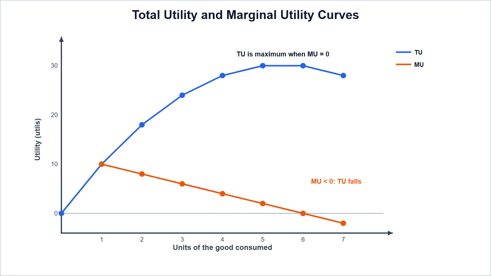
Remember: when MU is positive TU rises; when MU = 0 TU is maximum (point of satiety); when MU is negative TU falls.
Numerical 1: Calculate MU from the TU schedule: 10, 18, 24, 28, 30, 30, 28 utils for 1 to 7 units.
Given: TU1 to TU7 = 10, 18, 24, 28, 30, 30, 28
Formula: MUn = TUn – TUn-1
Solution: MU1 = 10 – 0; MU2 = 18 – 10; … MU7 = 28 – 30
Answer: MU = 10, 8, 6, 4, 2, 0, -2; MU diminishes and becomes negative after satiety.
Consumer’s equilibrium (one good): a consumer buys a good up to the point where MUx / Px = MU of money (or MUx = Px when utility is expressed in rupees). For two goods, the condition is MUx/Px = MUy/Py = MU of money (law of equi-marginal utility).
Numerical 2: MU of successive units of good X is 10, 8, 6, 4, 2 utils. Price of X is ₹2 and MU of one rupee is 2 utils. How many units will the consumer buy?
Given: MUx = 10, 8, 6, 4, 2; Px = ₹2; MUm = 2 utils
Formula: Buy while MUx/Px ≥ MUm
Solution: MUx/Px = 5, 4, 3, 2, 1; it equals MUm = 2 at the 4th unit
Answer: 4 units
Derivation of demand (cardinal): if Px falls, MUx/Px becomes greater than MUm, so the consumer buys more units until equality is restored. Thus quantity demanded rises when price falls.
2.1.2 Ordinal Utility Analysis
Ordinal analysis assumes utility can only be ranked (first, second, third preference), not measured. It uses indifference curves.
- Consumer’s bundle: a combination of two goods (x1, x2).
- Indifference curve (IC): a curve joining all bundles that give the consumer the same satisfaction, so the consumer is indifferent between them.
- Indifference map: a family of ICs; a higher IC represents a higher level of satisfaction (monotonic preferences: more is preferred to less).
- Marginal rate of substitution (MRS): the rate at which a consumer is willing to give up good 2 for one more unit of good 1 while staying on the same IC. MRS = ΔX2 / ΔX1 (absolute value) = slope of the IC.
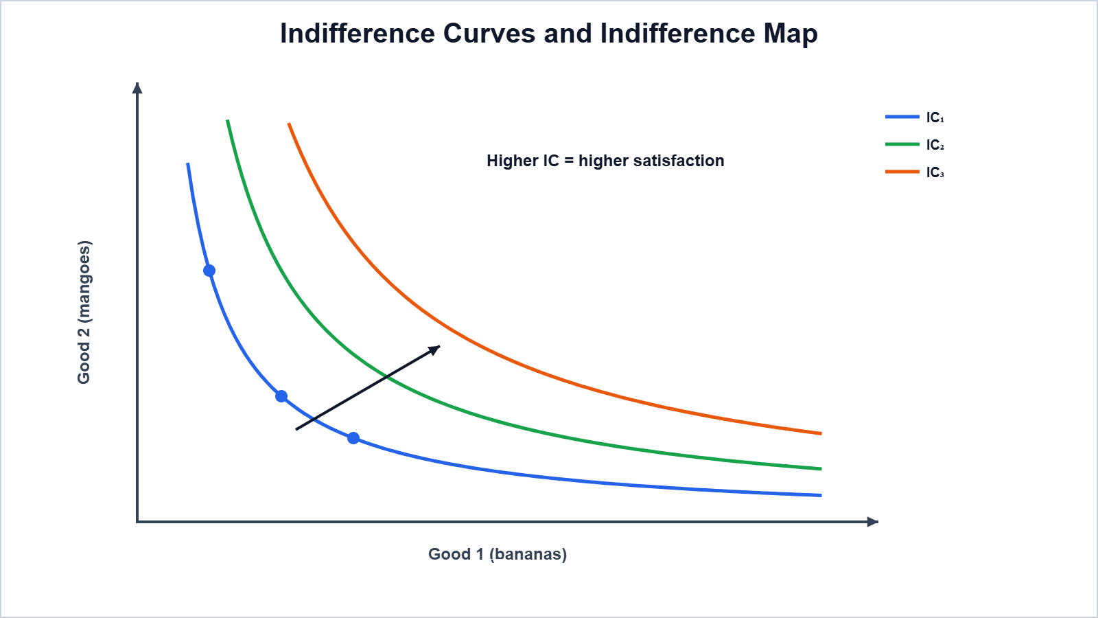
Properties of indifference curves: (1) they slope downward from left to right; (2) they are convex to the origin because of diminishing MRS; (3) higher ICs give higher satisfaction; (4) two ICs never intersect.
Bundle | Bananas (x1) | Mangoes (x2) | MRS |
|---|---|---|---|
A | 1 | 15 | – |
B | 2 | 11 | 4 |
C | 3 | 8 | 3 |
D | 4 | 6 | 2 |
E | 5 | 5 | 1 |
Numerical 3: Calculate MRS from the IC schedule above. What does it show?
Given: Bundles (1,15), (2,11), (3,8), (4,6), (5,5)
Formula: MRS = ΔX2 given up / ΔX1 gained
Solution: A→B: 4/1; B→C: 3/1; C→D: 2/1; D→E: 1/1
Answer: MRS = 4, 3, 2, 1: it is diminishing, so the IC is convex to the origin.
2.2 The Consumer’s Budget
2.2.1 Budget Set and Budget Line
A consumer can buy only those bundles whose cost does not exceed income. The budget set is the collection of all bundles that cost less than or equal to income: p1x1 + p2x2 ≤ M. The budget line shows bundles that cost exactly M: p1x1 + p2x2 = M.
Intercepts: M/p1 on the x1 axis and M/p2 on the x2 axis. Slope = -p1/p2 (the price ratio, i.e., the rate at which the market allows good 2 to be exchanged for good 1).
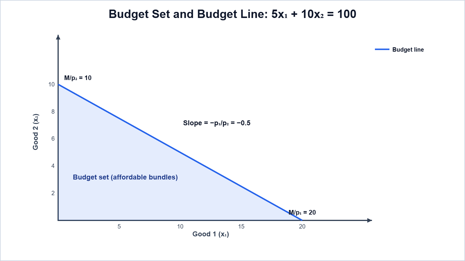
Numerical 4: A consumer has income ₹100. Price of good 1 is ₹5 and of good 2 is ₹10. Write the budget line equation, find the intercepts and the slope.
Given: M = 100; p1 = 5; p2 = 10
Formula: p1x1 + p2x2 = M; intercepts M/p1, M/p2; slope = -p1/p2
Solution: 5x1 + 10x2 = 100; 100/5 = 20; 100/10 = 10; slope = -5/10
Answer: 5x1 + 10x2 = 100; intercepts 20 units of good 1 and 10 units of good 2; slope = -0.5
2.2.2 Changes in the Budget Set
- Change in income: with prices constant, a rise in income shifts the budget line outward parallel; a fall shifts it inward. The slope does not change.
- Change in price of good 1: with income and p2 constant, a fall in p1 rotates the budget line outward around the x2 intercept (it becomes flatter); a rise rotates it inward.
- A change in p2 rotates the line around the x1 intercept.
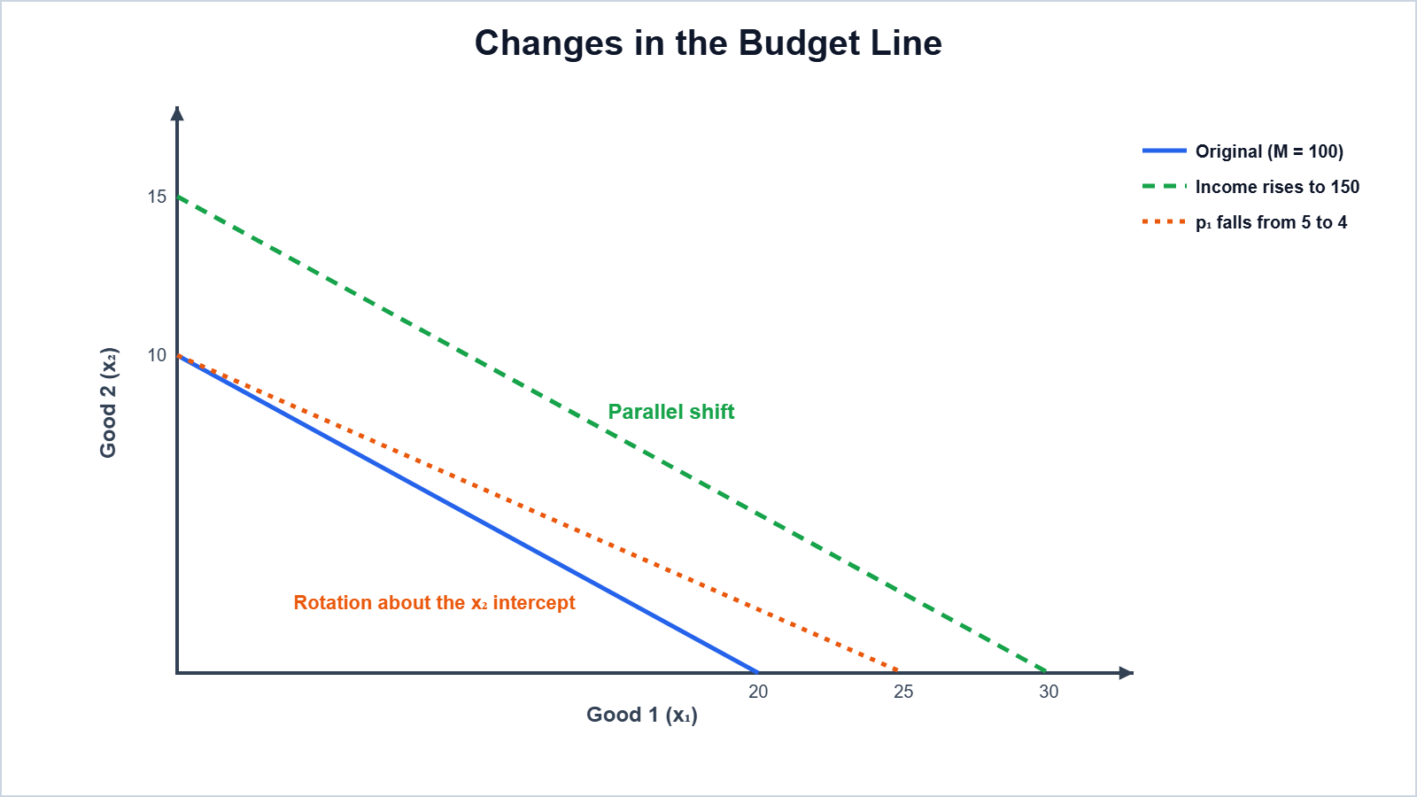
Numerical 5: In Numerical 4, find the new intercepts and slope if (a) income rises to ₹150; (b) p1 falls to ₹4 (income ₹100).
Given: (a) M = 150, p1 = 5, p2 = 10; (b) M = 100, p1 = 4, p2 = 10
Formula: Intercepts M/p1, M/p2; slope -p1/p2
Solution: (a) 150/5 = 30, 150/10 = 15, slope -0.5; (b) 100/4 = 25, 100/10 = 10, slope -4/10
Answer: (a) 30 and 15, slope -0.5 (parallel shift); (b) 25 and 10, slope -0.4 (rotation)
2.3 Optimal Choice of the Consumer
A rational consumer chooses the bundle on the highest attainable indifference curve. This happens where the budget line is tangent to an IC, i.e., where MRS = p1/p2, and MRS diminishes at that point.
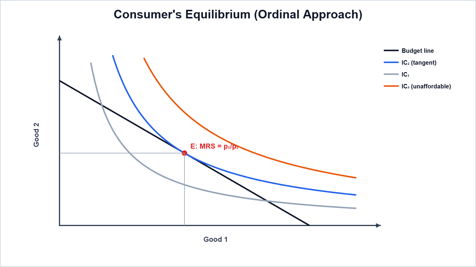
If MRS > p1/p2, the consumer values good 1 more than the market price, so buys more of good 1; if MRS < p1/p2, buys less of it, until equality is reached.
Numerical 6: Using the IC schedule in Numerical 3, p1 = ₹2, p2 = ₹1 and income = ₹14. Which bundle is optimal?
Given: MRS between C and D = 2; p1/p2 = 2/1; M = 14
Formula: Equilibrium: MRS = p1/p2, and the bundle lies on the budget line
Solution: At D (4, 6): cost = 2 x 4 + 1 x 6 = 14 = M, and MRS (C to D) = 2 = p1/p2
Answer: Bundle D: 4 bananas and 6 mangoes
2.4 Demand
Demand is the quantity of a good a consumer is willing and able to buy at a given price during a period of time. The demand function is q = d(p), showing how demand depends on price, other factors (income, prices of related goods, tastes) remaining constant.
2.4.1 Demand Curve and the Law of Demand
Law of Demand: other things remaining unchanged, there is an inverse relationship between the price of a good and its quantity demanded. The demand curve therefore slopes downward. A linear demand curve can be written as d(p) = a – bp.
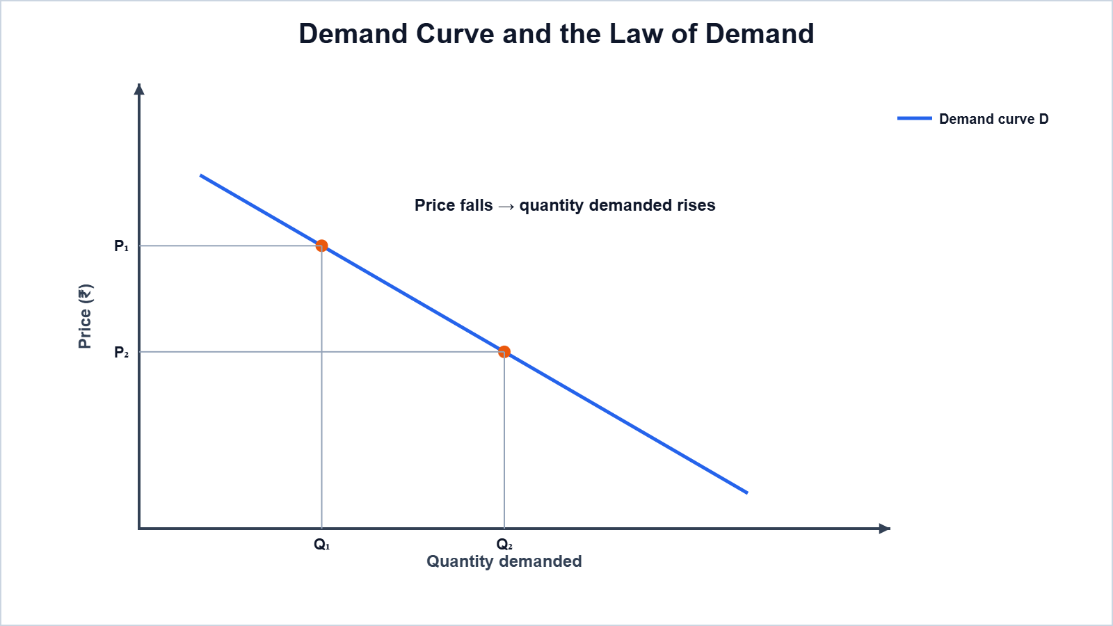
Reasons for the law: diminishing marginal utility; substitution effect (the good becomes relatively cheaper than substitutes); income effect (a fall in price raises real income).
2.4.2 Deriving a Demand Curve from Indifference Curves and Budget Constraints
When p1 falls, the budget line rotates outward and the consumer reaches a new tangency point on a higher IC, usually with more of good 1. Plotting each price of good 1 against the optimal quantity chosen gives the demand curve for good 1.
2.4.3 Normal and Inferior Goods
Normal good: demand rises with income (e.g., good-quality food, clothes). Inferior good: demand falls as income rises (e.g., coarse grains for a consumer who shifts to better food). A good can be normal at low income and inferior at high income.
2.4.4 Substitutes and Complements
Substitutes are used in place of each other (tea and coffee): a rise in the price of one raises the demand for the other. Complements are used together (pen and ink, car and petrol): a rise in the price of one reduces the demand for the other.
2.4.5 Shifts in the Demand Curve
The demand curve shifts when factors other than own price change. Rightward shift (increase in demand): rise in income (normal goods), rise in price of a substitute, fall in price of a complement, favourable tastes, expected price rise, larger population. The opposite changes cause a leftward shift (decrease).
2.4.6 Movements along the Demand Curve and Shifts in the Demand Curve
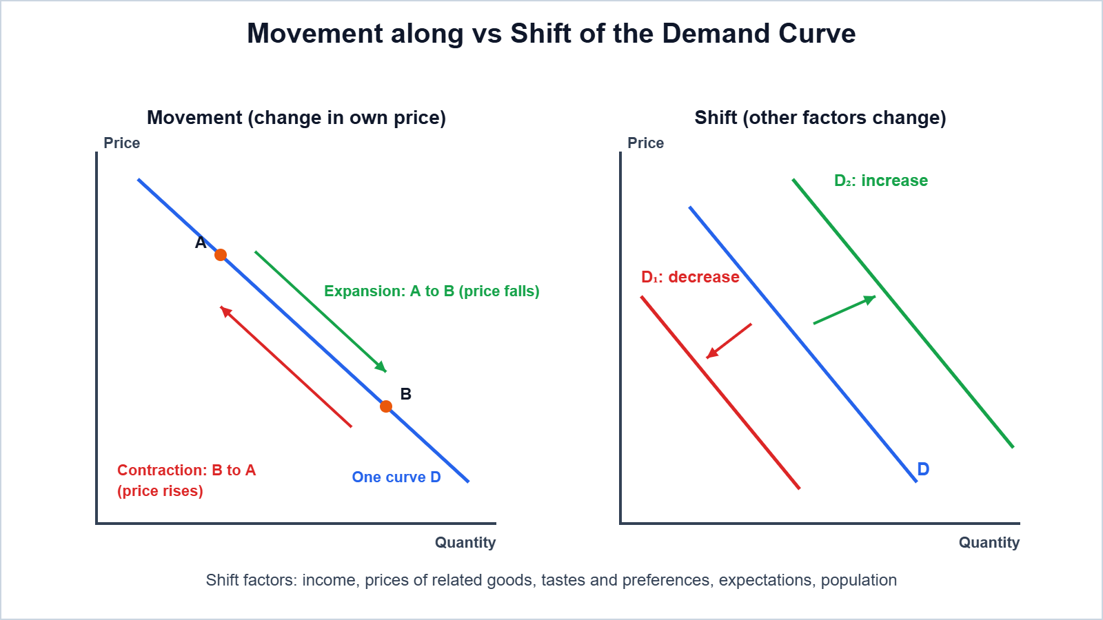
Movement along the curve | Shift of the curve |
|---|---|
Caused by change in the own price of the good | Caused by change in other factors (income, related prices, tastes) |
Expansion (price falls) or contraction (price rises) | Increase (rightward) or decrease (leftward) |
Same demand curve | New demand curve |
2.5 Market Demand
Market demand is the sum of the quantities demanded by all consumers at each price. Graphically, the market demand curve is the horizontal summation of individual demand curves.
Numerical 7: Find the market demand from the individual schedules: at prices ₹1, 2, 3, 4, consumer A demands 10, 8, 6, 4 and consumer B demands 8, 6, 4, 2 units.
Given: qA = 10, 8, 6, 4; qB = 8, 6, 4, 2
Formula: Market demand = qA + qB at each price
Solution: 10 + 8; 8 + 6; 6 + 4; 4 + 2
Answer: Market demand = 18, 14, 10, 6 units at prices ₹1, 2, 3, 4
2.6 Elasticity of Demand
Price elasticity of demand (eD) measures the responsiveness of quantity demanded to a change in the price of the good:
eD = (Percentage change in quantity demanded) / (Percentage change in price) = (ΔQ/Q) / (ΔP/P) = (ΔQ/ΔP) x (P/Q). Its value is negative because of the law of demand; we usually compare the absolute value.
Numerical 8: Price of a good falls from ₹5 to ₹4 and quantity demanded rises from 100 to 150 units. Find eD by the percentage method.
Given: P = 5, P1 = 4, Q = 100, Q1 = 150
Formula: eD = %ΔQ / %ΔP
Solution: %ΔQ = (50/100) x 100 = 50%; %ΔP = (-1/5) x 100 = -20%; eD = 50/(-20)
Answer: eD = -2.5; |eD| = 2.5, elastic demand
Numerical 9: When price rises from ₹10 to ₹12, quantity demanded falls from 50 to 40 units. Find eD.
Given: P = 10, ΔP = +2, Q = 50, ΔQ = -10
Formula: eD = (ΔQ/ΔP) x (P/Q)
Solution: eD = (-10/2) x (10/50) = -5 x 0.2
Answer: eD = -1 (unitary elastic)
Numerical 10: eD of a good is -2. Its price rises by 10%. If the consumer was buying 100 units, how much will be bought now?
Given: eD = -2; %ΔP = +10%; Q = 100
Formula: %ΔQ = eD x %ΔP
Solution: %ΔQ = -2 x 10 = -20%; new Q = 100 – 20% of 100
Answer: 80 units
2.6.1 Elasticity along a Linear Demand Curve
For a linear demand curve q = a – bp, eD = -bp/(a – bp), so elasticity is different at every point even though the slope is constant. Geometric (point) method: eD at a point = lower segment / upper segment of the demand curve. At the mid-point eD = 1; above it eD > 1; below it eD < 1; at the price axis eD = ∞; at the quantity axis eD = 0.
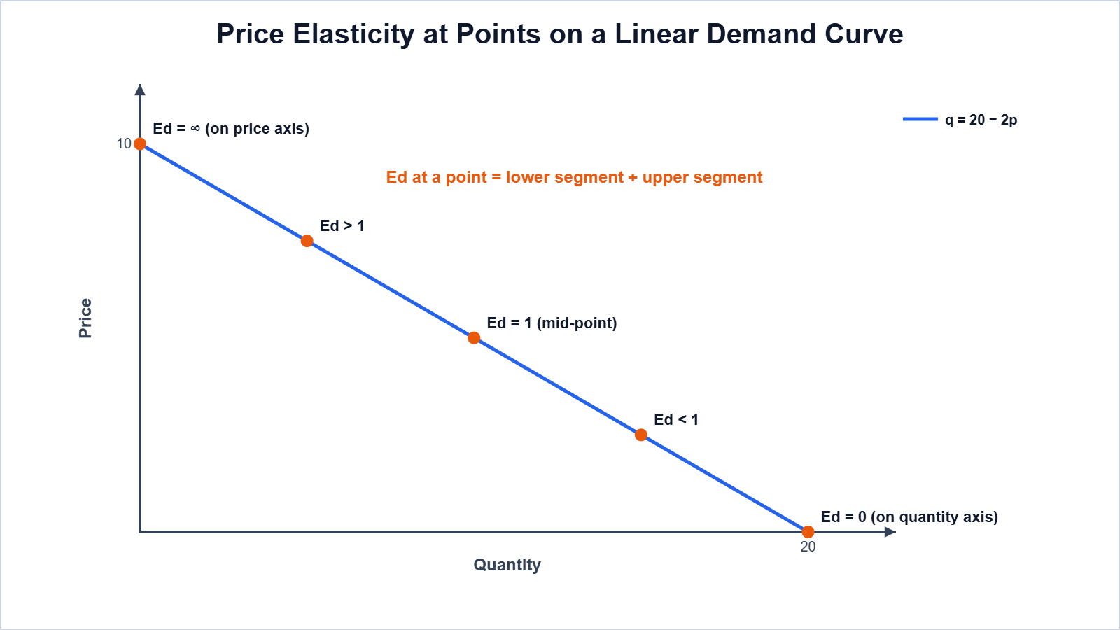
Numerical 11: For the demand curve q = 20 – 2p, find eD at p = 4 by the formula and by the geometric method.
Given: a = 20, b = 2, p = 4, so q = 20 – 8 = 12. Price intercept = 10
Formula: eD = -bp/q; geometric: lower segment / upper segment
Solution: Formula: -2 x 4/12 = -0.667. Geometric: along the price axis, lower part = 4 – 0 = 4 and upper part = 10 – 4 = 6, so 4/6
Answer: |eD| = 0.67 by both methods (inelastic)
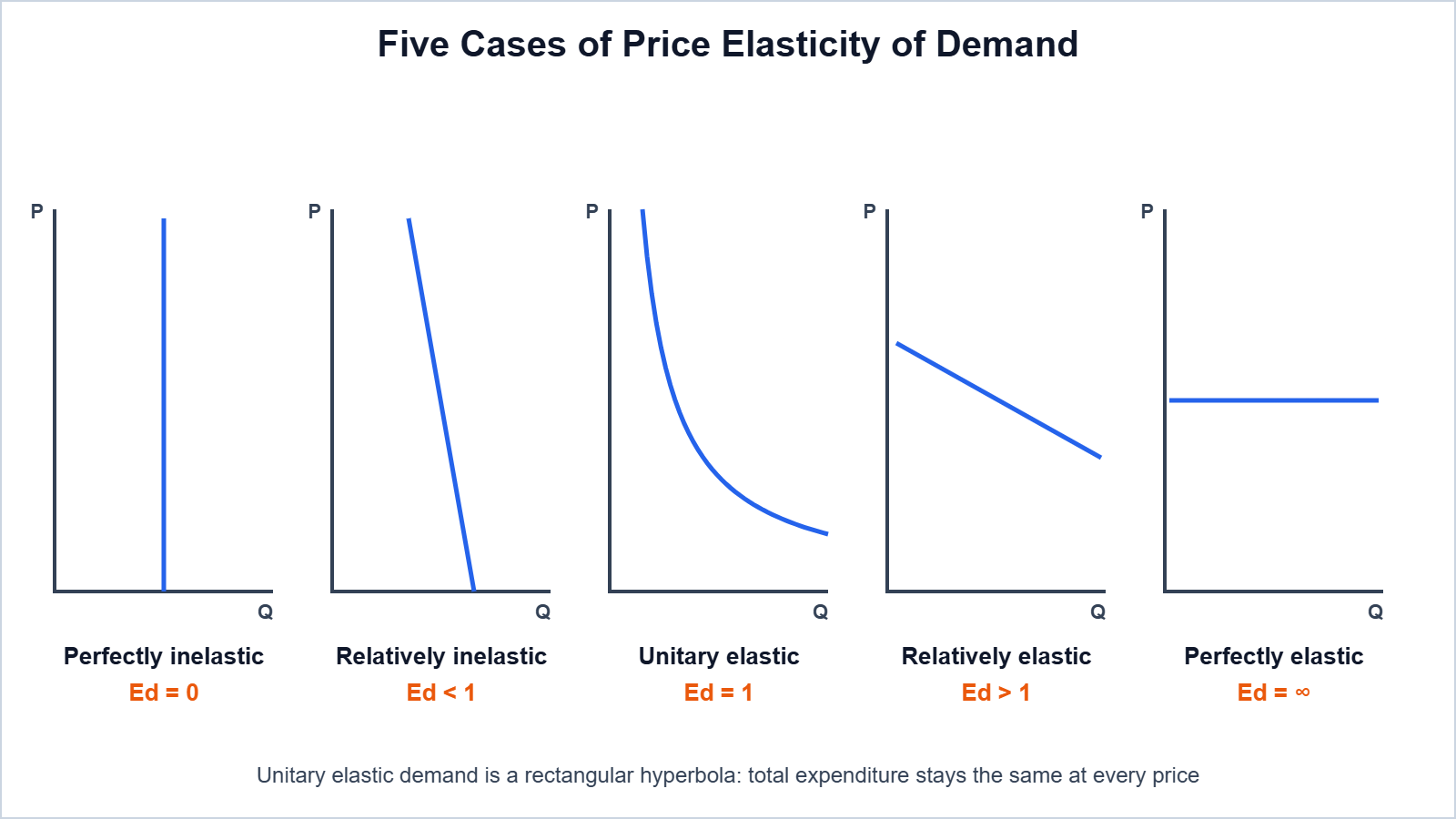
Case | Value | Shape of demand curve |
|---|---|---|
Perfectly inelastic | eD = 0 | Vertical |
Relatively inelastic | 0 < eD < 1 | Steep |
Unitary elastic | eD = 1 | Rectangular hyperbola |
Relatively elastic | eD > 1 | Flat |
Perfectly elastic | eD = ∞ | Horizontal |
2.6.2 Factors Determining Price Elasticity of Demand for a Good
- Nature of the good: necessities are inelastic; luxuries are elastic.
- Availability of close substitutes: more substitutes, more elastic.
- Share of income spent: goods taking a small share of income (salt, matchbox) are inelastic.
- Number of uses: goods with many uses (electricity) are more elastic.
- Time period: demand is more elastic in the long run.
- Habits: goods of habitual consumption are inelastic.
2.6.3 Elasticity and Expenditure
Total expenditure (outlay) method: expenditure = p x q.
Price change | Total expenditure | Elasticity |
|---|---|---|
Price falls | Rises | Elastic (eD > 1) |
Price falls | Unchanged | Unitary (eD = 1) |
Price falls | Falls | Inelastic (eD < 1) |
Numerical 12: Price falls from ₹5 to ₹4 and quantity rises from 100 to 150. Find the nature of elasticity by the total expenditure method.
Given: P = 5, Q = 100; P1 = 4, Q1 = 150
Formula: TE = P x Q
Solution: TE before = 5 x 100 = ₹500; TE after = 4 x 150 = ₹600
Answer: TE rises when price falls, so demand is elastic (eD > 1), which agrees with Numerical 8.
Easy Memory Trick: “Price and expenditure move opposite → Elastic; same direction → Inelastic; no change → Unitary”.
Practice Problems (Answers Only)
- Price rises from ₹20 to ₹25, quantity falls from 100 to 90. Find eD. Ans: -0.4 (inelastic)
- TU is 15, 27, 36 utils for 1, 2, 3 units. Find MU. Ans: 15, 12, 9
- M = ₹60, p1 = ₹3, p2 = ₹6. Find intercepts and slope of the budget line. Ans: 20 and 10; -0.5
- Price falls from ₹10 to ₹8, quantity rises from 20 to 25. Nature of elasticity by total expenditure method? Ans: TE stays ₹200, unitary elastic
- At the mid-point of a linear demand curve, what is eD? Ans: 1
Important Questions
Q1. State the law of diminishing marginal utility.
Ans. As more units of a good are consumed, the MU from each successive unit declines.
Q2. What is the relation between TU and MU?
Ans. TU rises when MU is positive, is maximum when MU is zero and falls when MU is negative.
Q3. Define an indifference curve. Why is it convex to the origin?
Ans. A curve of bundles giving equal satisfaction; it is convex because MRS diminishes.
Q4. Why can two indifference curves not intersect?
Ans. The intersection point would give two different levels of satisfaction at once, which is a contradiction.
Q5. Write the equation and slope of the budget line.
Ans. p1x1 + p2x2 = M; slope = -p1/p2.
Q6. State the conditions of consumer equilibrium in the ordinal approach.
Ans. MRS = p1/p2, and MRS must be diminishing at the point.
Q7. Distinguish between normal and inferior goods.
Ans. Demand for a normal good rises with income; for an inferior good it falls with income.
Q8. Distinguish between a movement along and a shift of the demand curve.
Ans. Movement is due to own price change; shift is due to change in other factors.
Q9. Why does elasticity differ along a straight-line demand curve?
Ans. Because the ratio P/Q changes at every point although the slope is constant.
Q10. State four factors affecting price elasticity of demand.
Ans. Nature of good, availability of substitutes, share of income spent and time period.
Conclusion: A rational consumer maximises satisfaction within the budget, where MU per rupee is equal (cardinal) or MRS equals the price ratio (ordinal). This choice gives a downward-sloping demand curve, whose responsiveness to price is measured by elasticity of demand.