Production and Costs – Class 12 Economics Notes
Part A: Introductory Microeconomics
Chapter – 3
Production and Costs
3.1 Production Function
Production is the process of converting inputs (labour, capital, land, raw materials) into output. The production function shows the technical relationship between physical inputs and the maximum output that can be produced with them: q = f(L, K), where L is labour and K is capital. It assumes a given state of technology.
Example: a farmer using 2 workers and 1 hectare of land can produce at most 10 quintals of wheat; the production function tells the maximum output for each combination of inputs.
3.2 The Short Run and the Long Run
Short run | Long run |
|---|---|
At least one input (usually capital) is fixed | All inputs are variable |
Output changed only by changing variable inputs | Output changed by changing all inputs (scale of production) |
Firm cannot change its plant size | Firm can change plant size; new firms can enter and old ones exit |
Studied through the law of variable proportions | Studied through returns to scale |
Remember: short run and long run are not fixed calendar periods; they depend on whether all inputs can be varied.
3.3 Total Product, Average Product and Marginal Product
3.3.1 Total Product (TP): the total output produced with a given quantity of the variable input, other inputs fixed. It is also called total physical product or total return to the variable input.
3.3.2 Average Product (AP): output per unit of variable input: APL = TPL / L.
3.3.3 Marginal Product (MP): the change in total product from using one more unit of the variable input: MPL = ΔTP / ΔL = TPL – TPL-1. Also, TP = sum of MPs.
Labour (L) | TP | AP = TP/L | MP = ΔTP/ΔL |
|---|---|---|---|
1 | 10 | 10 | 10 |
2 | 24 | 12 | 14 |
3 | 36 | 12 | 12 |
4 | 44 | 11 | 8 |
5 | 48 | 9.6 | 4 |
6 | 48 | 8 | 0 |
7 | 44 | 6.29 | -4 |
Numerical 1: From the TP schedule 10, 24, 36, 44, 48, 48, 44 for L = 1 to 7, calculate AP and MP.
Given: TP1 to TP7 as given
Formula: AP = TP/L; MP = TPL – TPL-1
Solution: AP: 10/1, 24/2, 36/3, 44/4, 48/5, 48/6, 44/7. MP: 10 – 0, 24 – 10, 36 – 24, 44 – 36, 48 – 44, 48 – 48, 44 – 48
Answer: AP = 10, 12, 12, 11, 9.6, 8, 6.29; MP = 10, 14, 12, 8, 4, 0, -4
Numerical 2: The MP of labour for the first four units is 5, 7, 6 and 4. Find TP and AP.
Given: MP = 5, 7, 6, 4
Formula: TPL = ΣMP; AP = TP/L
Solution: TP: 5; 5 + 7 = 12; 12 + 6 = 18; 18 + 4 = 22. AP: 5/1, 12/2, 18/3, 22/4
Answer: TP = 5, 12, 18, 22; AP = 5, 6, 6, 5.5
3.4 The Law of Diminishing Marginal Product and the Law of Variable Proportions
Law of diminishing marginal product: if we keep increasing the use of one input while other inputs are fixed, a point is eventually reached after which the marginal product of that input starts falling.
Law of variable proportions: when more and more units of a variable input are combined with a fixed input, the marginal product of the variable input first rises and then falls (and may become negative). The name comes from the changing proportion of variable to fixed input.
Reasons: MP rises at first because the fixed input is underused and better division of labour becomes possible; it falls later because each extra unit of the variable input gets less of the fixed input to work with; it becomes negative when there is overcrowding.
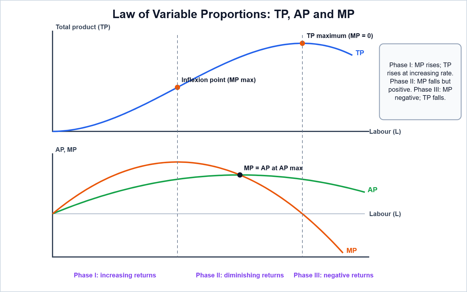
Phase | TP | MP | AP |
|---|---|---|---|
I: Increasing returns to a factor | Rises at an increasing rate | Rises | Rises |
II: Diminishing returns to a factor | Rises at a diminishing rate, reaches maximum | Falls, but positive; becomes zero when TP is maximum | Falls after reaching maximum (where MP = AP) |
III: Negative returns to a factor | Falls | Negative | Falls but stays positive |
Exam point: A rational producer operates in Phase II, where MP is falling but positive.
3.5 Shapes of Total Product, Marginal Product and Average Product Curves
- The TP curve first rises at an increasing rate (convex), then at a decreasing rate (concave) after the point of inflexion, reaches a maximum and then falls.
- The MP and AP curves are inverse U-shaped.
- Relation between AP and MP: when MP > AP, AP rises; when MP = AP, AP is at its maximum; when MP < AP, AP falls. The MP curve cuts the AP curve from above at the maximum of AP.
- Relation between TP and MP: TP rises when MP is positive, is maximum when MP = 0 and falls when MP is negative.
Easy Memory Trick: “MP leads, AP follows”: MP rises first, peaks first and falls first.
3.6 Returns to Scale
In the long run all inputs can be changed together. Returns to scale show how output changes when all inputs are increased in the same proportion.
Type | Meaning | Example: all inputs doubled |
|---|---|---|
Increasing returns to scale (IRS) | Output increases in a greater proportion | Output more than doubles |
Constant returns to scale (CRS) | Output increases in the same proportion | Output exactly doubles |
Decreasing returns to scale (DRS) | Output increases in a smaller proportion | Output less than doubles |
For a Cobb-Douglas production function q = LαKβ: α + β > 1 gives IRS; α + β = 1 gives CRS; α + β < 1 gives DRS.
Numerical 3: For q = L0.5K0.5, find output when L = K = 4 and when L = K = 8. Identify the returns to scale.
Given: α = 0.5, β = 0.5; inputs doubled from 4 to 8
Formula: q = L0.5K0.5 = √(LK)
Solution: q = √(4 x 4) = 4; q = √(8 x 8) = 8
Answer: Output doubles from 4 to 8: constant returns to scale (α + β = 1)
Numerical 4: For q = 2L0.6K0.6, by what factor does output rise when both inputs are doubled?
Given: α + β = 0.6 + 0.6 = 1.2
Formula: New q / old q = 2α + β
Solution: 21.2
Answer: Output rises about 2.30 times: increasing returns to scale
3.7 Costs
Cost function: shows the minimum cost of producing each level of output, given input prices. Costs include payments to hired inputs (explicit costs) and the imputed value of the firm’s own inputs (implicit costs, including normal profit).
3.7.1 Short Run Costs
- Total fixed cost (TFC): cost of fixed inputs; does not change with output and is incurred even at zero output (rent, interest, salary of permanent staff). Its curve is horizontal.
- Total variable cost (TVC): cost of variable inputs; changes with output and is zero at zero output (raw materials, wages of casual labour).
- Total cost (TC) = TFC + TVC.
- Average fixed cost: AFC = TFC/q; it falls continuously as output rises (rectangular hyperbola) and never touches the axes.
- Average variable cost: AVC = TVC/q; U-shaped.
- Short run average cost: SAC = TC/q = AFC + AVC; U-shaped.
- Marginal cost: MC = ΔTC/Δq = ΔTVC/Δq (fixed cost does not change); U-shaped. Also, TVC = ΣMC.

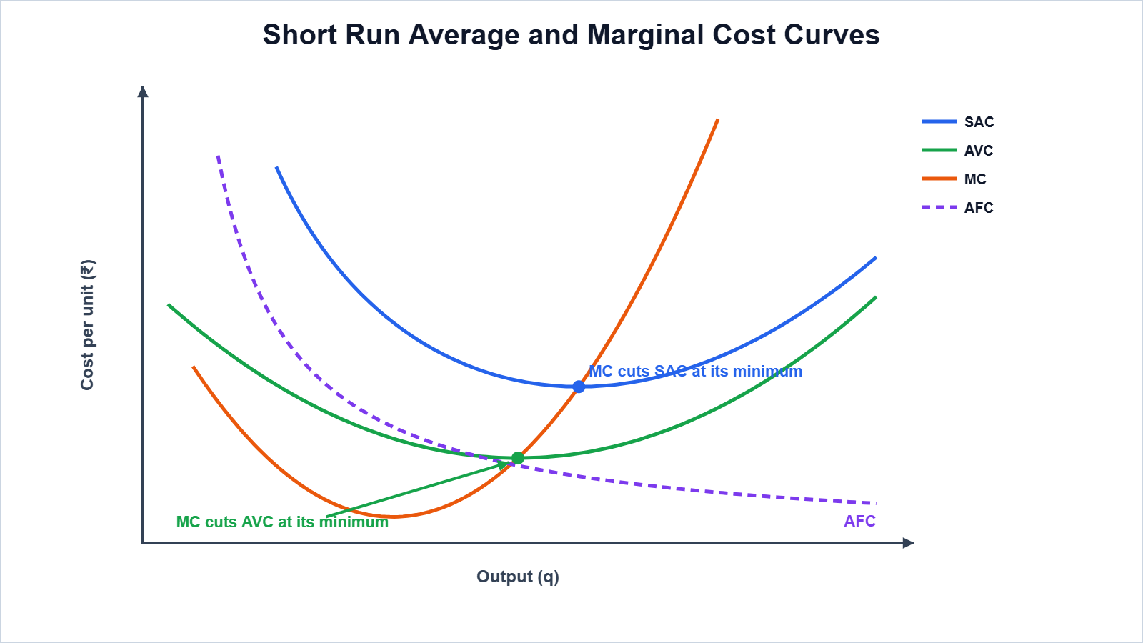
Why are AVC, SAC and MC U-shaped? Because of the law of variable proportions: when MP of the variable input rises, the cost of producing each extra unit falls, and when MP falls, it rises. Relationships: MC cuts AVC and SAC at their minimum points from below; the gap between SAC and AVC (= AFC) narrows as output rises; minimum AVC occurs at a lower output than minimum SAC.
q | TFC | TVC | TC | AFC | AVC | AC | MC |
|---|---|---|---|---|---|---|---|
0 | 60 | 0 | 60 | – | – | – | – |
1 | 60 | 20 | 80 | 60 | 20 | 80 | 20 |
2 | 60 | 36 | 96 | 30 | 18 | 48 | 16 |
3 | 60 | 48 | 108 | 20 | 16 | 36 | 12 |
4 | 60 | 64 | 124 | 15 | 16 | 31 | 16 |
5 | 60 | 90 | 150 | 12 | 18 | 30 | 26 |
6 | 60 | 126 | 186 | 10 | 21 | 31 | 36 |
Numerical 5: TFC = ₹60 and TVC for 1 to 6 units = 20, 36, 48, 64, 90, 126. Calculate TC, AFC, AVC, AC and MC.
Given: TFC = 60; TVC as given
Formula: TC = TFC + TVC; AFC = TFC/q; AVC = TVC/q; AC = TC/q; MC = TCq – TCq-1
Solution: e.g., at q = 4: TC = 60 + 64 = 124; AFC = 60/4 = 15; AVC = 64/4 = 16; AC = 124/4 = 31; MC = 124 – 108 = 16
Answer: See the table above. AVC is minimum (16) at 3-4 units and AC is minimum (30) at 5 units; MC is minimum (12) at 3 units.
Numerical 6: TC of a firm is ₹50, 80, 100, 115, 140 at output 0, 1, 2, 3, 4. Find TFC, TVC, MC and AVC.
Given: TC at q = 0 is ₹50
Formula: TFC = TC at zero output; TVC = TC – TFC; MC = ΔTC; AVC = TVC/q
Solution: TFC = 50; TVC = 30, 50, 65, 90; MC = 30, 20, 15, 25; AVC = 30/1, 50/2, 65/3, 90/4
Answer: TFC = ₹50; TVC = 30, 50, 65, 90; MC = 30, 20, 15, 25; AVC = 30, 25, 21.67, 22.5
Numerical 7: TFC of a firm is ₹120. Find AFC at outputs 1, 2, 3, 4 and show that AFC x q is constant.
Given: TFC = 120
Formula: AFC = TFC/q
Solution: 120/1, 120/2, 120/3, 120/4; each AFC x q = 120
Answer: AFC = 120, 60, 40, 30; AFC x q = TFC = 120 always, so the AFC curve is a rectangular hyperbola.
3.7.2 Long Run Costs
In the long run all costs are variable, so there is no fixed cost: LRTC = LRTVC. Long run average cost: LRAC = LRTC/q; long run marginal cost: LRMC = ΔLRTC/Δq.

- The LRAC curve is U-shaped due to returns to scale: IRS (economies of scale) make LRAC fall, CRS make it flat, DRS (diseconomies of scale) make it rise.
- LRAC is an envelope of the SAC curves: it touches each SAC curve at one point, showing the lowest cost of producing each output when plant size can be chosen.
- LRMC cuts LRAC at its minimum point from below; LRMC is also U-shaped.
Practice Problems (Answers Only)
- TP rises from 25 to 30 when labour rises from 4 to 5. Find MP and AP at L = 5. Ans: MP = 5; AP = 6
- TVC at q = 2 is ₹20 and at q = 3 is ₹45. Find MC of the 3rd unit. Ans: ₹25
- AFC at 5 units is ₹12. Find TFC and AFC at 6 units. Ans: ₹60; ₹10
- When all inputs are increased by 10%, output rises by 15%. Name the returns to scale. Ans: Increasing returns to scale
- If q = L0.4K0.4, what are the returns to scale? Ans: Decreasing (α + β = 0.8; doubling inputs raises output about 1.74 times)
Important Questions
Q1. What is a production function?
Ans. The technical relation between inputs and the maximum output: q = f(L, K).
Q2. Distinguish between short run and long run.
Ans. In the short run some inputs are fixed; in the long run all inputs are variable.
Q3. Define TP, AP and MP.
Ans. TP is total output; AP = TP/L; MP = change in TP from one more unit of the variable input.
Q4. State the law of variable proportions.
Ans. With a fixed input, as more variable input is used, MP first rises and then falls, possibly becoming negative.
Q5. Explain the relation between AP and MP.
Ans. AP rises when MP > AP, is maximum when MP = AP and falls when MP < AP.
Q6. What are returns to scale? Name their types.
Ans. Change in output when all inputs change proportionately: IRS, CRS and DRS.
Q7. Why does the AFC curve never touch the x-axis?
Ans. TFC is positive, so TFC/q can never become zero however large q is.
Q8. Why are AVC and MC curves U-shaped?
Ans. Because of the law of variable proportions (MP first rises and then falls).
Q9. Explain the relation between MC and AC.
Ans. When MC < AC, AC falls; when MC = AC, AC is minimum; when MC > AC, AC rises.
Q10. Why is the LRAC curve called an envelope curve?
Ans. It envelops the SAC curves, touching each at one point.
Conclusion: The production function links inputs to output. In the short run the law of variable proportions shapes TP, AP and MP and makes cost curves U-shaped; in the long run returns to scale shape the LRAC curve.